by Davis Foote, Daylen Yang, Mostafa Rohaninejad
In recent years, numerous results have shown that state-of-the-art convolutional models for image classification learn to represent meaningful and human-interpretable features that indicate a level of semantic understanding of the image content (see DeepDream, neural style, etc.). However, work in this direction has in large part remained confined to the domain of images. Until only recently, little attention had been given in the deep learning community to the potential of adapting these ideas to the domain of raw audio. WaveNet is a recently proposed autoregressive model that learns to generate audio at the sample level with a clever architecture that can train on sequential data in parallel. Its generated samples are promising and show that it is within our reach to model the intricacies and long-term dependencies that audio requires. With these two fields of background work in mind, we set off to try to understand what kinds of features and latent representations our models can learn for working with raw audio.
Our motivating application is adapting the neural style algorithm to work on audio. This problem is motivating from a research-oriented perspective for the reasons discussed in the previous paragraph. Style transfer has also found commercial interest as a way of one-shot learning filters for photography.

Given a sufficiently sophisticated audio style transfer system, the same framework can be adapted as a tool for musicians: to emulate processed vocals from a song on the radio, for example, you need only record a short example clip, then mix this as the “style” target with a recording of your own voice as the “content” target.

We had not realized how ambitious this was in reality. As discussed above, little to no work has been done to understand what kinds of features these models learn to represent audio signals. This work is necessarily evaluated subjectively, as are most similar results even in the more well-understood domain of images. Our experimentation in attempting to directly adapt the known algorithms to work in this other domain led us to the conclusion (which we will defend later in this report) that achieving the aforementioned goals will require substantial novel work in understanding how this type of data fundamentally differs from images.
Thus we restate our goal: we hope to create a meaningful and interpretable latent space model for raw audio that can be used as a baseline for future work in this domain. This is not so vague a goal as it sounds: a good latent space model should encode semantics so that perturbations in latent space correspond to human-interpretable changes in the content or style of the corresponding raw audio. Ideally, each dimension in latent space should encode an orthogonal semantic component of the information in an audio signal. In essence, we seek to find and describe the low-dimensional manifold corresponding to natural signals (we consider music and speech) embedded in the high-dimensional space of raw audio.

Approach
We divided our efforts into two approaches:
- Inspired by the original style transfer algorithm, we examine the layer activations of networks trained for classification and generation tasks.
- We used variational inference over latent variable models of audio generation.
We also briefly did some baseline work on a model that attempts to form style transfer without any learned filters, which we will briefly discuss.
Data
We used a number of datasets to train our models. For music, we turned to the MagnaTagATune dataset. This dataset contains about 20,000 30-second clips of audio (so about 160 hours total), and each clip is annotated with a set of tags such as “guitar,” “classical,” “slow,” “techno,” and so on. The audio files are in MP3 format.
For spoken English, we used the VCTK dataset. This dataset contains 109 different speakers, each reading out 400 sentences of English. The dataset contains many samples from both genders.
We also used the MNIST handwritten digits dataset to test our Variational Lossy Autoencoder.
Baseline
Work from the signal processing community suggests that time-domain representations of waveforms (that is, raw audio) are not as interpretable as frequency-domain representations. Our first approach started from this mindset: that the style and content information we seek might be visible in the spectral properties of the data. Inspired by the neural style algorithm, our algorithm was thus as follows:
- Let
and
be the short-time Fourier transforms of the target content signal and style signal, respectively.
- Use a first-order optimization method to find a matrix X that minimizes
, where
is
loss.
- Return
, the inverse short-time Fourier transform of
.
Supposing that the STFT is a meaningful featurization of the data, the “content loss” 


Unfortunately, this differs from the neural style algorithm in one key way: the style features here are drawn from small enough receptive fields that this Gram matrix fails to encode the local statistics we care about and simply incentivizes certain frequency bands playing consistently throughout the output signal.
Concretely, when we run this algorithm with
We used Librosa, an open-source Python library, for out-of-the-box short-time Fourier transform and inverse short-time Fourier transform implementations.
Network Activations
We used two different models here: WaveNet and a vanilla 1-D convolutional neural network classifier.
WaveNet
We started with an existing open-source implementation of WaveNet. To describe our algorithm, there is some necessary background both on the neural style algorithm and WaveNet.
The neural style algorithm operates under the guiding principle that convolutional neural networks build increasingly abstract representations of their input as it passes deeper into the network. The core idea is that this means information about local statistics (“style information”) is encoded in the activations at shallower layers and information about global statistics (“content information”) is encoded in the activations at deeper layers. Thus the style and content of two images can be blended by optimizing over input images which match the respective (shallow and deep) layer activations of the two targets. They improve upon this on the style matching side by discarding spatial information beyond the receptive field of the style layer activations. This is done by taking correlations of each filter response and combining them into the Gram matrix G. This ensures that the information that the input tries to match encodes only local textures rather than global arrangement.
In the original paper and most variants published afterward, the architecture to which this algorithm is applied is some VGGNet variant. Our first goal was to see how directly this could be ported to work with WaveNet.
At the level of abstraction we are interested in, the architecture for WaveNet can be summarized as in the following diagram:

For a more detailed description of the various blocks in this diagram (1 x 1, Dilated Conv, Causal Conv), please refer to the WaveNet paper. Here we focus on the residuals and the Softmax distribution at the output. We use the residuals (the element-wise sum of the 1×1 conv and the output from the previous residual block) because these are most analogous to the normal convolutional layers in VGGNet.
So this leaves us with a clear algorithm: pre-train a WaveNet on some dataset, pick a deep layer and a shallow layer (or set of shallow layers), and apply the neural style algorithm on the outputs of the residuals. However, there is one major problem with this: WaveNet as described in the paper and implemented in the repo linked above discretizes the input signal and takes the one-hot encoding of each sample’s discretized value (out of 256 possible values). The input to the network is thus a 256 x T matrix, where T is the number of samples in our waveform, and each slice at a particular time index is a one-hot vector. The outputs of the network are interpreted as the log odds for each potential value of the sample conditioned on the values of the previous samples. If we backpropagate gradients of some loss function to the input, we end up with a matrix of shape 256 x T full of real numbers, which cannot be directly transformed into a concrete audio signal.
The probabilistic interpretation of these numbers is that the vector corresponding to each sample was optimized conditioned on distributions of neighboring samples, and we are left with log odds for marginal distributions on each sample at the input. We believe, but have not yet formalized, that this is analogous to performing max-product belief propagation on the following semi-Markov chain graph according to clique potentials dictated in some way by WaveNet and the loss functions we are attempting to optimize.
The issue is that this has discarded conditional information between different samples. If we take the maximum likelihood value per audio sample to reconstruct a signal, then each marginal audio sample has been optimized, but in no way do we have a jointly likelihood-maximizing signal. Indeed, results from attempting this method were only white noise.
Our goal is to end up with a 256 x T matrix where each time-indexed sliced is a one-hot vector so that we can simply invert WaveNet’s discretization frontend and recover a meaningful signal. To this end, we perform coordinate gradient descent, only allowing a single sample to be modified at once. At convergence, we take the max-likelihood from the resulting softmax distribution and fix the vector to be a one-hot vector according to the chosen value. In this way, we incrementally build toward a convergent input matrix that globally optimizes our objective subject to the constraint that it can be inverted to obtain a signal. Under the probabilistic interpretation, this corresponds to a Gibbs-sampling like max likelihood procedure.
Unfortunately, TensorFlow was not particularly amenable to this algorithm. If we vectorize the input matrix to be a single tensor variable object, the optimizer interface does not allow us to specify that only certain indices can be trained at once. Thus we are forced to use a separate variable per time index. This results in an enormous graph—one second of audio at 16kHz sampling rate leads to 16,000 separate trainable tensors. We found this far beyond the scope of what could reasonably be run to convergence on modern hardware.
At this point, the uncertainty due to neural style not previously having been proved on a ResNet-like architecture and the apparent dead-end of our optimization procedure being too slow led us to instead consider a more straightforward architecture based on VGGNet.
1-D CNN Classifier
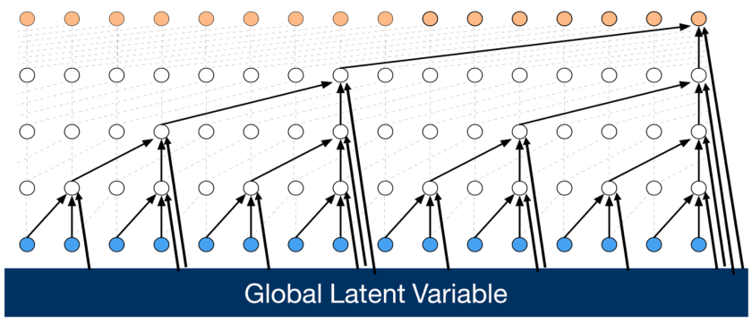
VGGNet takes in fixed-size raw images as input and produces a distribution over 1000 classes as the output. Its architecture is pretty straightforward—it’s a series of convolutional and pooling layers, followed by some fully connected layers. So we decided to try the same thing for audio: our network takes in a fixed size chunk of raw audio and predicts the tags that apply to the audio clip. It turns out that this has been tried before. We decided to replicate the architecture described in Dieleman’s paper, End-to-End Learning for Music Audio. The diagram below illustrates the architecture:

We did stray from Dieleman’s paper in a couple ways, however. We used Adam instead of SGD. We also performed tag merging on the MagnaTagATune dataset—using this helpful list of duplicate tags, we combined tags such as “male,” “male singer,” and “male vocal,” into a single tag. We also shuffled the data and used a 95-5% split ratio for the train and validation sets, as opposed to not shuffling the data and using the first 76% of the data for training as many existing papers do. Finally, we preprocessed the raw input audio signal to be between -1 and 1, with mean 0, while Dieleman uses the WAV file input (each sample is an integer between 0-65536).
The metric we used is average AUC over the top 50 tags. After 12 hours of training, our average AUC was 0.895 on our validation set. As we mentioned above, our validation set differs from the validation set that most other papers use; however, for rough comparison purposes, other average AUCs we have seen on this task are 0.888 (Deep-BoF), 0.849 (Dieleman’s model), and 0.882 (Dieleman’s model with extra features).
We also have some qualitative examples! Here’s what our model came up with for these popular songs:
- “Shake It Off” by Taylor Swift: rock, guitar, drum
- “You’ve Got A Friend In Me” by Randy Newman: guitar, vocal, male
- “i hate u, i love u” by gnash, Olivia O’Brien: guitar, vocal, female
- “This Is What You Came For” by Calvin Harris, Rihanna: techno, beat, vocal, drum, fast, electro
- “Time” by Hans Zimmer: slow, ambient, quiet
Equipped with this classifier, we then tried a couple experiments to see if we could perform style transfer:
- “Image Fooling”: Initialize a signal at the input of the network as some starting audio (e.g. a clip of music) and maximize a particular output or the activations at a particular layer. All results sounded like white noise added to the initial clip.
- Neural Style: Simultaneously try to match activations at a deep layer with one clip and temporal correlations (in order to eliminate indexical temporal information) of activations at a set of layers with another clip. Results again sounded like white noise mixed with content clip.
Discussion of these results is deferred to the “Lessons Learned” section.
Our code for our audio classifier, along with a pre-trained model, is available here.
Variational Inference
The other approach we have followed in order to learn a meaningful latent space is to assume a probabilistic latent variable model. Consider the following generative model for a dataset
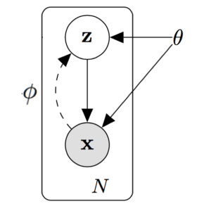
Latent variables 


To deal with the intricacies of raw audio data, we would like to use WaveNet to model the conditional distribution. The original WaveNet paper describes a gating mechanism for conditioning WaveNet on latent variables; the modified model and our implementation are detailed in a later section (see “Conditional WaveNet” below).
Unfortunately, such powerful models tend to get stuck in local optima in which the KL divergence penalty in the evidence lower bound is driven to zero and the posterior encodes no information. The Variational Lossy Autoencoder is a proposed solution to this problem, in which limiting the decoder’s expressivity to only modeling local statistics forces the posterior to learn to model global dependencies. Concretely, for audio this is done by using an unusually shallow WaveNet that gives conditional distributions based on a relatively small receptive field, so that any influence on a sample from past samples beyond that receptive field can only be modeled in the latent code.
We found that existing open-source TensorFlow implementations of the variational auto-encoder were not sufficiently general to be used as a variational lossy autoencoder; all assume that the distribution of interest is image structured and that the decoder is a Gaussian distribution parameterized by some neural network. (As a more speculative point of commentary, it seems that there are no implementations whatsoever of the algorithm in its full generality; all implementations are specific to some project.) We thus created our own implementation. Additionally, no open-source implementation of WaveNet supported conditioning, so we added this functionality to the WaveNet repository linked above.
Variational Autoencoder
Our implementation of the VAE and code to reproduce the original VAE MNIST results are available at https://github.com/djfoote/audio-style-transfer/tree/master/vae. Sample digits are included here. Higher quality samples can be generated by running the training script from our repo to convergence.

We implemented the necessary features of the VAE for it to be used as a VLAE as mentioned in the previous paragraph. The VLAE algorithm requires a sophisticated autoregressive decoder, so in order to have demonstrable visual results with images, we would have needed e.g. a PixelCNN implementation that can plug in to our VAE. We determined that we did not have the cycles to implement this solely for the purpose of illustrating the VLAE algorithm. Instead we proceed directly to Conditional WaveNet implementation.
Unfortunately, there has been a lot of confusion surrounding how to structure the conditional WaveNet interface to be used by the VAE implementation, and we were unable to get this training procedure working in time for this report. However, we believe that, somewhat orthogonally to our original goals, our general open-source VAE implementation and our conditional WaveNet implementation have their own individual merit.
Conditional WaveNet
The WaveNet model can be tweaked to allow for Global and Local Conditioning. Global Conditioning variables are temporally invariant features describing the input that the network has available to it during training. These variables are conditioned on at every node. This makes the equation come out in a different form.

Local Conditioning allows for temporally variant features that form a time series, often at a much lower frequency than the input. Therefore, the Local Conditioning variables are normally up-sampled so to match the sampling frequency of the input. Alongside global conditioning, it allows for some compelling results. In the original paper they attained state of the art text to speech.

We found the method described in the original paper to model these conditional in-dependencies to be powerful[WN].

Where 


Since we have our results from using global conditioning on speaker and we do not condition on time aligned words or linguistic features, the end result is garble. However, our global conditioning has been proved to work: the garble can be toggled to be distinctly male or female!
Male garble:
Female garble:
Lessons Learned
At heart, our goal is to add momentum to recent work using modern deep learning developments to raw audio and to use these methods to better understand this complex type of data. On this level we draw one main conclusion: audio is dissimilar enough from images that we shouldn’t expect work in this domain to be as simple as changing 2D convolutions to 1D.
We have seen that nearly every single operation which we expected to be semantically meaningful based on our experience in computer vision has led to changes that sound like nothing more than noise to the human ear. Consider the resolution at which humans typically process auditory information. For music, even a well-trained ear typically does not process anything lower-level than “the alto saxophone is playing a C# and the piano is playing an A major chord”. For speech, people primarily translate the audio into an internal language model, and beyond that process stylistic information such as speaker identity and tempo. This suggests that within the space of 16kHz sampled audio clips collected over several seconds, the manifolds corresponding to music and speech are both extremely low-dimensional. Perhaps these somewhat arbitrary transformations in the space of network layer activations (see image fooling and neural style experiments for our audio classifier) bring us into audio space lying off the music and speech manifolds so that the model has learned nothing in this region and we truly do just get white noise.
We believe that the probabilistic direction holds promise as a solution to this problem. In this setting, we are explicitly performing nonlinear dimensionality reduction in a principled way so that interpolations and other operations in latent space correspond to movement along the manifold we are interested in. We are excited to continue pursuing this avenue of research in the future.
On a more personal level, this project was an amazing opportunity to learn a lot about signal processing, working with TensorFlow, and understanding the dirtiest details of reimplementing published models.
Team Contributions
After an excruciatingly detailed accounting of the work done by our team, we determined that the exact percentage breakdown per person is:
- Davis: 34.33%
- Daylen: 33.33%
- Mostafa: 32.33%
Davis: Designed and implemented baseline model. Implemented neural style for both WaveNet and VGG-like audio classifier. Fleshed out probabilistic interpretation of WaveNet results; came up with MCMC max-likelihood/coordinate descent algorithm to rectify results. Read a lot of papers to try to come up with promising directions. Came up with VLAE approach (latent variable model with conditional WaveNet as decoder) and implemented VAE. Wrote sections of presentation/poster/report corresponding to these contributions, and wrote additionally wrote introduction and conclusion sections to final report. Came up with dope blog post title.
Daylen: Trained WaveNet on the VCTK dataset to be used for the neural style algorithm. Implemented a 1-D convolutional model for audio classification and trained it on the MagnaTagATune dataset. Experimented with optimizing with respect to the input audio signal in order to maximally activate output style units. Contributed to the presentation, poster, and final blog post. Made sweet Kanye West and Taylor Swift graphic.
Mostafa: Implemented Conditional Wavenet and produced reasonable results with global conditioning. Refactored the repo to allow it work seamlessly with the MagnaTagATune dataset. To facilitate future work, added text to the input pipeline using Glove embedding. (Currently text can only be treated as a global conditioning variable which is not interesting, but whenever a dataset with time aligned words appears, we can easily incorporate it). Contributed to the creation of the powerpoint, poster, and final blog post, and attended all the corresponding events.
